
Plugin usage#
Tutorial#
A detailed tutorial can be found at Demo
Plugin Steps#
Open a 3D + time raw image and optionally its segmentation image, mask image in the viewer or select the provided sample data from the Napari menu.
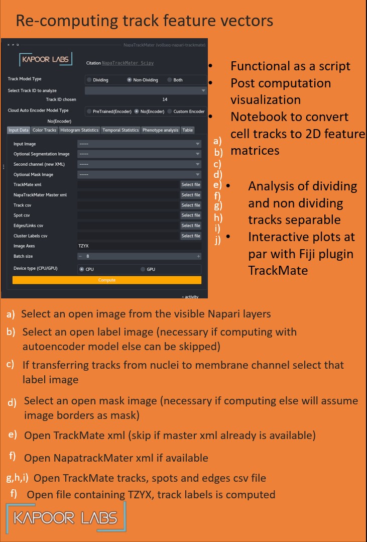
Launch the plugin and select the raw and segmentation image, provide the paths for xml and csv files.
If you want to create master xml file select a pre-trained autoencoder model or load a .ckpt file if you have trained one using our lightning library.
Click the compute tracks button.
Wait for computation to be over, the progress of different steps is displayed in the progress bar.
Once done you can view the histogram, mean-variance, phenotype plots and a track table.
You can interactively select the track anaylsis type to be dividing or non-dividing, that will update the plots too.
You can selet a TrackMate track id to visualize the tracks or you can select to visualize all tracks.
Tracks can be colored using different track properties or if segmentation image is also input into the plugin you can color that image with chosen track and spot attributes.
Segmentation and Tracking#
VollSeg has multiple model combinations for obtaining segmentations, some of its combination are more suited for certain image and microscopy types, the details of whcih can be found in the VollSeg repository. The output of segmentation are instance labels for 2D, 3D, 2D + time, and 3D + time datasets. The aim of obtaining these labels is accurate quantification of cell shapes as that is usually a biological aim for researchers interested in cell fate quantification and this tool was made as a Napari grant action to achieve that purpose in cell tracking.
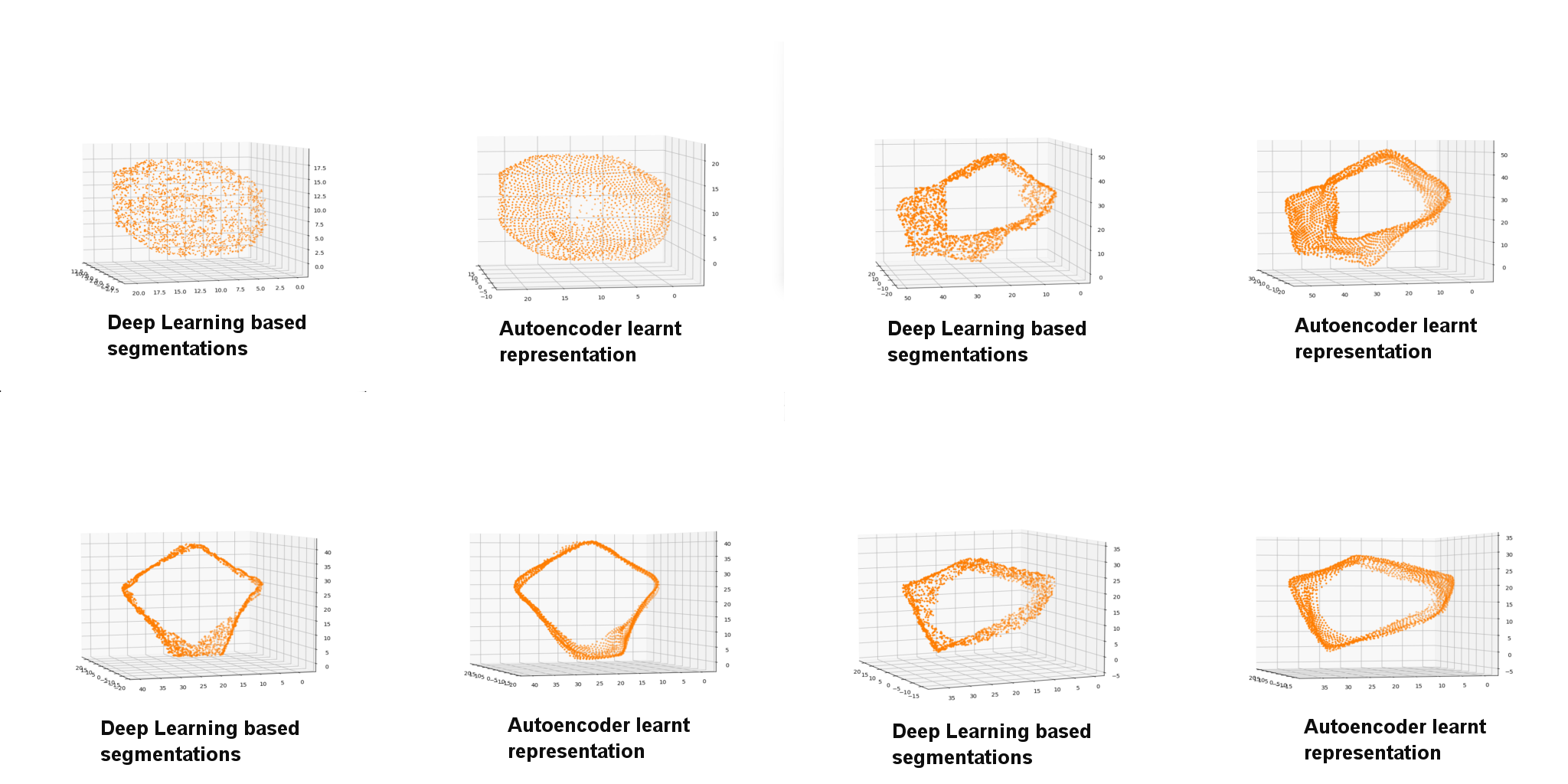
In our algorithm we train an autoencoder model to obtain point cloud representation of the segmentation labels (figure below).
In our algorithm the segmentation labels coming from VollSeg along with Raw image of the cells and tissue boundary mask of those cells serve as an input to this plugin. The tracking is performed prior to using this plugin in Fiji using TrackMate, which is the most popular tracking solution with track editing tools in Fiji. The output of that plugin are xml and [tracks, spots and edges csv files] that serve as an input to this plugin. We also provide pre-trained auto encoder models for nuclei and membrane that can be used to obtain the point cloud representation of the segmented cells. The users can also provide their own autoencoder models if they have trained them on their data.
Point Clouds#
As a first step the users apply the trained autoencoder models on the input timelapse of segmentation and in the plugin point cloud representation of all the cells in the tracks are computed. We provide a script to visualize point cloud representation for the input segmentation image (binary) using classical and autoencoder model predictions.
Autoencoder#
This is an algorithm developed by Sentinal AI startup of the UK and they created a pytorch based program to train autoencoder models that generate point cloud representations. KapoorLabs created a Lightning version of their software that allows for multi-GPU training. In this plugin autoencoder model is used to convert the instances to point clouds, users can select our pre-trained models or choose their own prior to applying the model. The computation is then performed on their GPU (recommended) before further analysis is carried out. As this is an expensive computation we also provide a script to do the same that can be submitted to the HPC to obtain a master XML file that appends additional shape and dynamic features to the cell feature vectors therby enhancing the basic XML that comes out of TrackMate.
Auto Track Correction#
We use a mitosis and apoptosis detection network to find the locations of cell sin mitosis which is then used as prior information to solve a local Jaqman linker for linking mitotic cell trajectories and terminating the apoptotic cell trajectories. To red more about this approach please read more about oneat
Shape Features#
The shape features computed in the plugin uses the point cloud representations produced by the autoencoder model. We compute the following shape features
Eccentricity
Eigenvectors and Eigenvalues of covariance matrix
Surface area and Volume
Dynamic Features#
The dynamic features computed in the plugin are the following
Radial Angle: Angle between the center of the tissue and the cell centroid taking the origin as top left co-ordinate of the image. demonstration
Motion Angle: Angle between the center of the tissue and the difference between the cell locations in successive co-ordinates.
Cell Axis Angle: Angle between the center of the tissue and largest eigenvector of the cell.
Speed: Cell speed at a given time-instance.
Acceleration: Cell acceleration at a given time-instance.
Distance of cell-mask: Distance between cell and the tissue mask at a given time-instance.